Great HVAC Meltdown
So two nights ago the heat went out in the middle of the night. Not super crazy- it’s been running 24/7 for almost two weeks.
I flipped the breakers. Didn’t change anything. Set the space heaters up in the bedroom and went back to sleep, thinking it was probably gonna be an easy fix.
Next morning I pop the air handler open and check- we’re getting voltages in the right spots. 240v, yep. But looks like a fuse popped.
Weirdly uses standard automotive fuses. I go try and steal one from the car, but it’s a 3A and the car doesn’t have any of those, so I get a pack from the auto store. Figuring poor, tired HVAC just blew ’cause it had been running forever.
Pop a new fuse in, turn the breakers back on, and the thermostat turns on for one SECOND then the fuse pops.
Take the thermostat off the wall and pop in a new fuse, turn everything back on – fuse does NOT pop. So — either the thermostat’s shot or something it was trying to turn on popped the fuse.
Start multimetering everything. Unplug the thermostat wires from the control board side on the air handler and FML- two of the wires are dead short to each other. How does this happen it’s not like I accidentally went under the house and put a nail through the wire.
Sooooo I need to run a new wire.
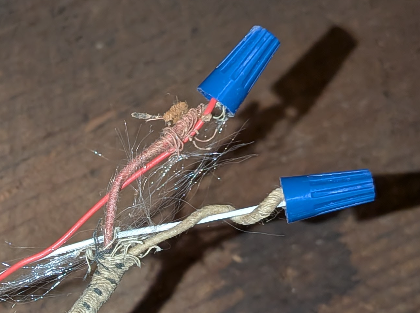
Which kinda checks out. When I put this new thermostat in a month ago or so, there was an ULTRA sketch wire in there that I’ve been affectionately calling “mummy wire.” Wire from the olden days, when you wrapped copper in cotton.
The thermostat I have needs six wires, and this mummy wire was being used instead of one of the six from the proper cable.
So I gotta run a new wire from the thermostat to the HVAC. Go to Lowe’s and buy some 18/7 (18-gauge, 7-conductor) wire, 50 feet. And I start pullin’ cable.
For the thermostat area, I can at least use the old wire as a pull cable. I tie some paracord to it and pull that into the crawl space, then I cut the old wire off the paracord and use the paracord to pull the 6 feet of cable or whatever back up into the wall. (Did it in that order so I didn’t have to pull 50 feet through the hole in the wall.)
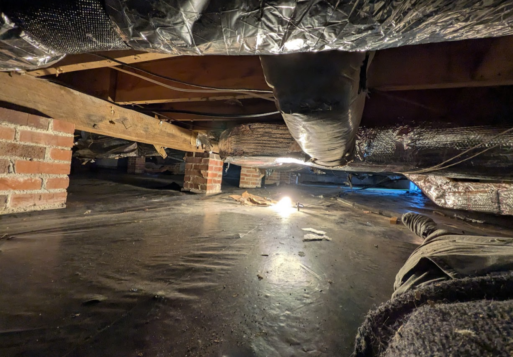
Crawl space is much less gross than average, with a pretty recent vapor barrier. But I get like 25 feet from the hatch and SOMETHIN’ SCUTTLIN’ ABOVE ME ON THE DUCTS.
I slide back to the next closest area with more headroom. Get my legs bent up so I can kick whatever is stalking me.
But the noise stops. My heart slows. I go back to pullin’ cable.
The back part of our house has a laundry room where the HVAC interior unit is- which, if you’re working on it, is nice ’cause it’s in conditioned space. But it seems there’s no access from under the house to the space under where the unit is, so I gotta figure out how to pull this cable into that room.
I trace the old cable, but it does something nuts. It goes up the wall on the opposite side of the room into the attic and down back to the air handler. I bought 50 feet of cable after measuring the run- thought I’d need 40 feet, but I don’t have enough to do that run. Also, pulling a cable through a full-height wall sucks.
So I start scuttlin’ back to the hatch to see what I can see from above.
And as I near the hatch-
I CATCH SOME MOTION BEHIND ME.
Somethin’ big just jumped up from the floor to the top of the duct. Stalking me.
I get out and figure out I can pull the cable through where the condensate drain runs. Get the fish tape down through there and, I think, into the crawl space. So I go back down to pull the cable with the fish tape and-
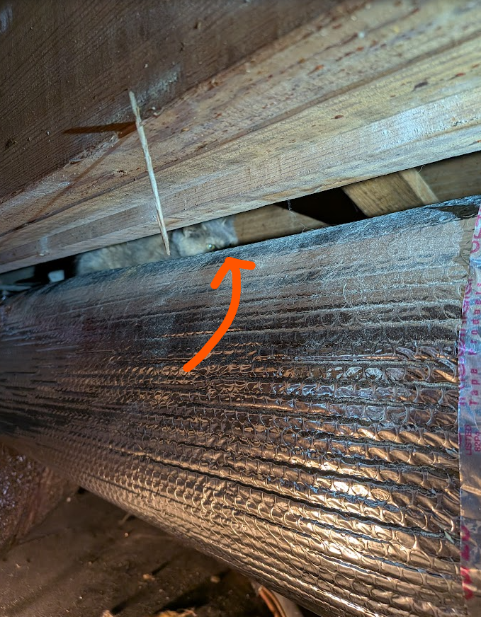
Find my stalker.
A FUCKING CAT.
Who also, presumably, butt-slammed some cable of the ancients and caused my current dead-short-problem.
I try to boop it off the top of the duct with one of those zip ties that Homeland Security and HVAC installers both use, but it’s not budging. So I go about my business. Connect the cable to the fish tape, then go up and finish pulling the cable to the air handler.
The house is now 55°F.
But there’s still the mummy cable to decipher. There’s no mummy cable in the air handler, so some asshole spliced it somewhere. And none of the wires in the air handler are labeled.
Mummy wire is a critical wire- it’s the reversing valve control wire. Tells the heat pump if it should make heat or cold, which we need heat right now.
I go digging around in the attic and find the mummy wire spliced into some 18/8, but WHICH 18/8 is it in the air handler? There are four.
I check continuity on yellow-black on one of the 18/8s and get nothing. Then I go back in the attic and strip and twist the yellow-black together next to the mummy wire. Recheck the continuity downstairs and it’s now continuous on yellow-black.
I have found my reversing valve wire.
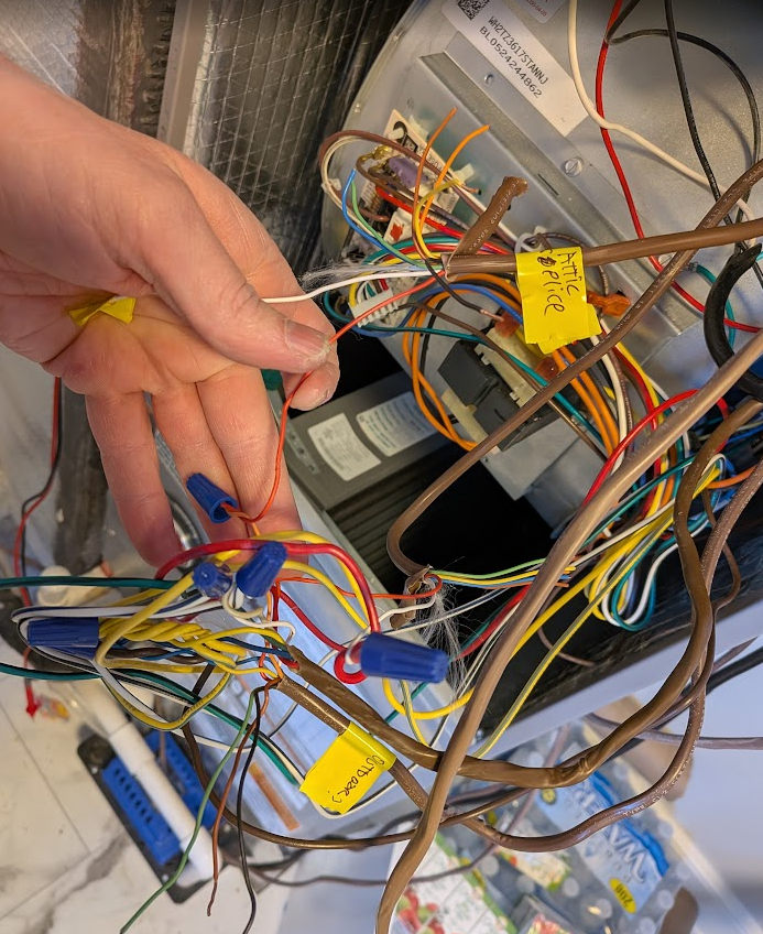
Then I can rewire and label the mess the previous monster left. Only half of the wires pictured.
I get everything reconnected, power on, testing voltages at the thermostat before I connect it and I get NOTHING on red-blue/C wires, which should be ~24V.
Turns out I over-twisted and work-hardened a red wire till it broke. Stripped and twisted that back on. And finally: ~24V red-blue/C.
Then the thermostat.
And the fuse did not pop.
And we have heat.
And I’m covered in disgusting cat fur from rolling around under the house for half the day.
Hit the Claude Code Limit?
I hit my Claude Code limit and needed to keep working my project using another LLM. If you use plan mode, Claude saves those plans and you can grab them and pass them into another LLM. Claude Code saves plan markdown files in two places:
./.claude/plans/~/.claude/plans/
The files have random names like gentle-gliding-bear.md, sort by timestamp or grep for words related to your current project!
Black and Decker Vacuum (CHV1410L) Repair 2026
I’ve had this little vacuum since 2019 (~7 years at the time I’m writing this).
I replaced the batteries a couple of years ago and more than doubled the runtime when it was new. I had to take the battery apart and weld new cells in, it’d be nice if they sold replacement batteries.
In the last few months, it’s started making a terrible squealing noise with no suction. The squeal will go away if I bump the vacuum really hard or turn it on and off several times in a row, but it’s been getting worse requiring more bumps or on/off cycles.
I finally got around to taking the vacuum apart again, and the brass bushings on the motor are shot. I suspect you could extend the life of the vacuum by putting some oil on the bushings once a year but mine are too far gone for that.
The motor is labeled:
Leshi Motor
LS-545PC-63483
14.4V
180120/C
I was not able to find that part number for sale anywhere.
Here are the dimensions of the motor:
- Motor diameter: 35.5mm
- Motor body length (not including shaft): 59mm
- Motor length overall (including shaft): 90mm
- Shaft length: 30mm
- Shaft diameter: 3.17mm (1/8″?)
- Mounting screw spacing at front near shaft: 25mm
The motor is apparently a standard size overall “rs-545”, but this motor has a very long shaft. It looks like most of the motors sold in this size have a ~8mm long shaft. I think you could JUST get away with using a motor that has a 15mm shaft, but 20-30mm would be better. This motor from eBay for ~$12 including shipping (vmotor v060268), has been working fine for a week in the vacuum.
I did drill a hole in the motor shroud so I could get to the end bearing without complete disassembly, I think the front bearings are JUST reachable with the shroud on. Hope this motor lasts at least as long as the first one did!
The Bridged Edition
Some years ago, I had a thought about abridged and unabridged books. I wondered what would happen if we took the abridged version and subtracted it from the unabridged one.
What would be left is a new thing. The “bridged” edition. All the words nobody wants.
I wrote some code and tried this with several books – but abridging involves too much rewriting, the diffs were nonsense.
I had read the British and American version of Harry Potter and wondered if there might be difference beyond the normal loo becoming toilet, jumper becoming sweater, and motorbike becoming motorcycle.
I wondered if the bridged book code would work here.
tldr; check out the US-UK comparisons.
Dean Thomas
I expected mostly small dialect changes. Then my script produced this:
| UK Version | US Version |
|---|---|
| And now there were only [three] people left to be sorted [] Turpin, Lisa” became a Ravenclaw and then it was Ron’s turn. | And now there were only [four] people left to be sorted [Thomas, Dean,” a black boy even taller than Ron, joined Harry at the Gryffindor table] Turpin, Lisa,” became a Ravenclaw and then it was Ron’s turn. |
That’s … strange.
This description of Dean Thomas appears only in the American version. Was it in the original manuscript and later cut in the UK? Did the US editors ask for it to be added? I do not know.
Update: I spent some more time searching and found this explanation:
This was an editorial cut in the British version; my editor thought that chapter was too long and pruned everything that he thought was surplus to requirements. When it came to the casting on the film version of ‘Philosopher’s Stone’, however, I told the director, Chris, that Dean was a black Londoner. In fact, I think Chris was slightly taken aback by the amount of information I had on this peripheral character. I had a lot of background on Dean, though I had never found the right place to use it. His story was included in an early draft of ‘Chamber of Secrets’ but then cut by me, because it felt like an unnecessary digression. Now I don’t think his history will ever make it into the books.
The Code
I wrote a pipeline to compare the books. Ebooks are messy, so I had to clean them up before I could diff them.
Here is what I used:
- Calibre: I used
ebook-convertto extract raw text from different ebook formats. - Normalization: I used
ftfyto fix Unicode problems. I also wrote regex rules for things like honorifics. The UK uses “Mr” while the US uses “Mr.”. - Comparison and ignoring: The tool walks through the books word by word. It checks a list of known dialect swaps and ignores pairs like “color” and “colour”, so the output is not flooded with spelling noise. I also used Double Metaphone. If two words sound the same, the script ignores them.
What Else Changed?
Here are a few odd changes among many:
Chamber of Secrets: Apparition Explanation
The US version adds a whole world-building segment that’s not in the UK version.
| UK Version | US Version |
|---|---|
| And even underage wizards are allowed to use magic if it’s a real emergency, section nineteen or something of the Restriction of Thingy…” [] Harry’s feeling of panic turned suddenly to excitement. “Can you fly it?” | And even underage wizards are allowed to use magic if it’s a real emergency, section nineteen or something of the Restriction of Thingy – ” [“But your mum and dad…” said Harry, pushing against the barrier again in the vain hope that it would give way. “How will they get home?” “They don’t need the car!” said Ron impatiently. “They know how to Apparate! You know, just vanish and reappear at home! They only bother with Floo powder and the car because we’re all underage and we’re not allowed to Apparate yet…”] Harry’s feeling of panic turned suddenly to excitement. “Can you fly it?” |
Chamber of Secrets: Lucius Malfoy’s Entrance
The US version gives Lucius Malfoy a rougher entrance. It explains why he looks disheveled – Dobby was wiping his shoes. The UK version cuts this context.
| UK Version | US Version |
|---|---|
| [This entire section is missing] | Apparently Mr. Malfoy had set out in a great hurry, for not only were his shoes half-polished, but his usually sleek hair was disheveled. Ignoring the elf bobbing apologetically around his ankles… |
Prisoner of Azkaban: Dementor Release
The US version is more explicit about the Dementor letting Harry go.
| UK Version | US Version |
|---|---|
| Facedown, too weak to move, sick and shaking, Harry opened his eyes. [] The blinding light was illuminating the grass around him. | Facedown, too weak to move, sick and shaking, Harry opened his eyes. [The dementor must have released him.] The blinding light was illuminating the grass around him. |
Deathly Hallows: The Ear Joke
There’s an ear-joke adjustment.
| UK Version | US Version |
|---|---|
| Not so fast, [Lugless] said Fred, and darting past the gaggle of middle-aged witches heading… | Not so fast, [Your Holeyness] said Fred, and darting past the gaggle of middle-aged witches heading… |
The Reports
I generated interactive reports for all seven books. I’ve left out all the Mom/Mum and Color/Colour changes but otherwise, you can use the filters to see the actual additions and removals.
- Book 1: The Sorcerer’s/Philosopher’s Stone
- Book 2: The Chamber of Secrets
- Book 3: The Prisoner of Azkaban
- Book 4: The Goblet of Fire
- Book 5: The Order of the Phoenix
- Book 6: The Half-Blood Prince
- Book 7: The Deathly Hallows
I am working on generalizing the code so I can use it for other comparisons soon. If you find any other odd differences in the reports, let me know.
Replacing the 'Non-Replaceable' Battery in the Tile Slim
I replaced the battery in my Tile Slim! It uses a little tiny pouch cell (Ultralife CP114951 3.1v 380mAh).
Be careful, this is going into scary lithium battery territory. I shaved the plastic from the edges of the Tile Slim until I could peel the plastic shell apart; if I were to do it again, I think that I would sand the edges using some 80 or 120 grit sandpaper. The pouch cell inside is protected by a thin sheet 0.0015″ (0.0381mm) of stainless-steel top and bottom that’s glued in.
After you get into the package, you’ll need to trim off a bit of the rubber around the pouch cell terminals. Trim the terminals as close to the edge of the pouch cell as possible without cutting the pouch cell, while also not shorting your scissors across the terminals!
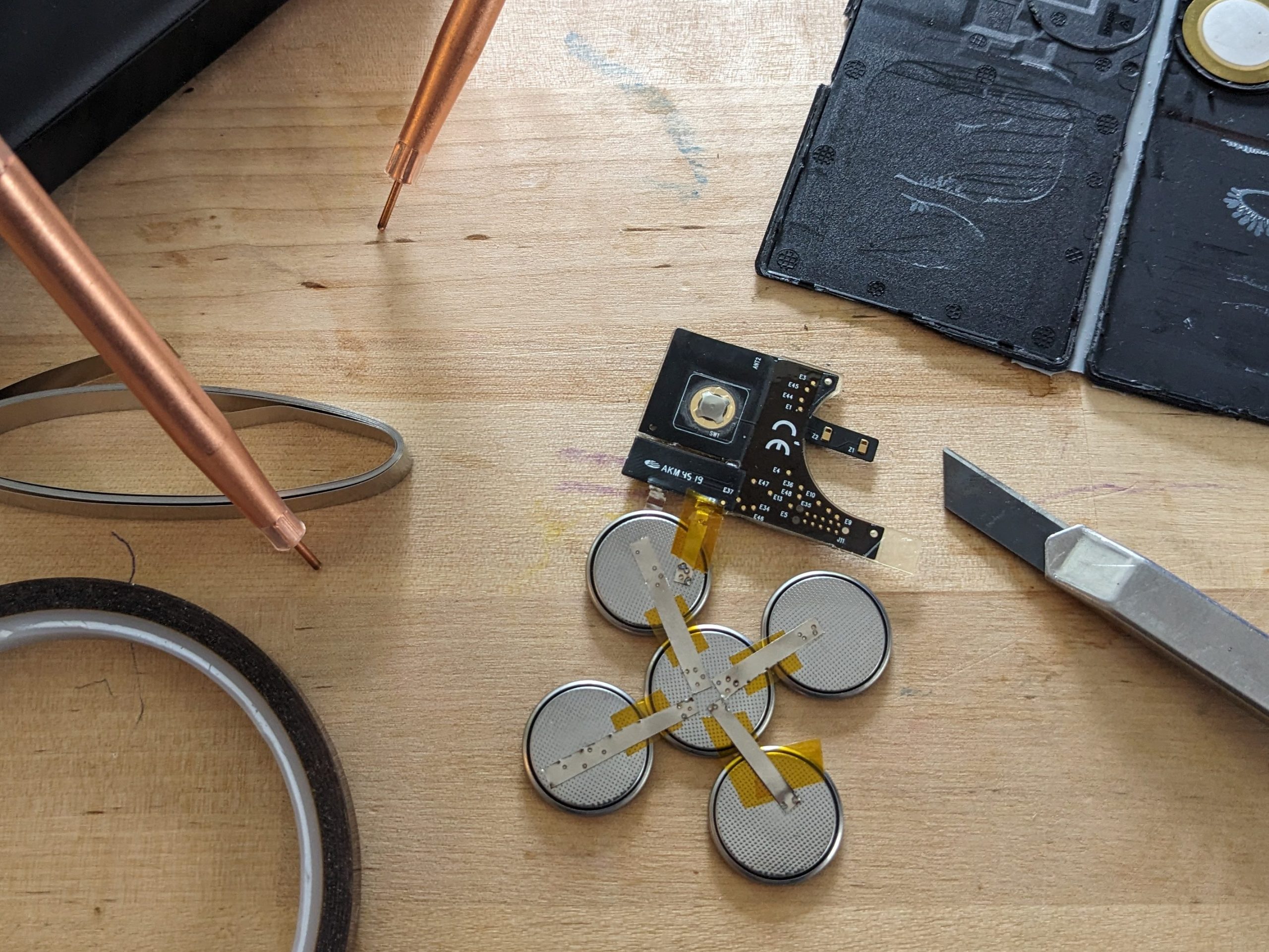
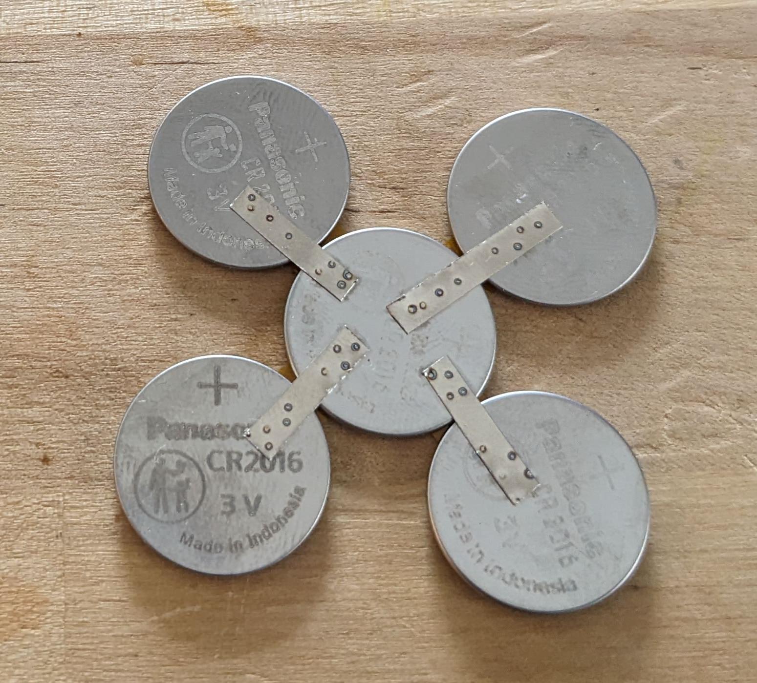
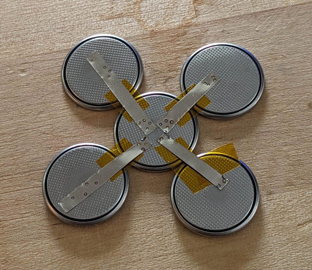
The pouch cell plus the stainless-steel plus the glue is about 0.0580″ (1.48mm). I wanted to stick close to that but figured going over a bit was ok. With a bit of measuring I figured out I could just fit five CR2016 0.787×0.0629″ (20×1.6mm) batteries in parallel in the case in a “X” configuration.
So, I got out the battery welder and cut some thin nickel strips and started welding. I applied some little strips of Kapton tape to make sure nothing shorted.
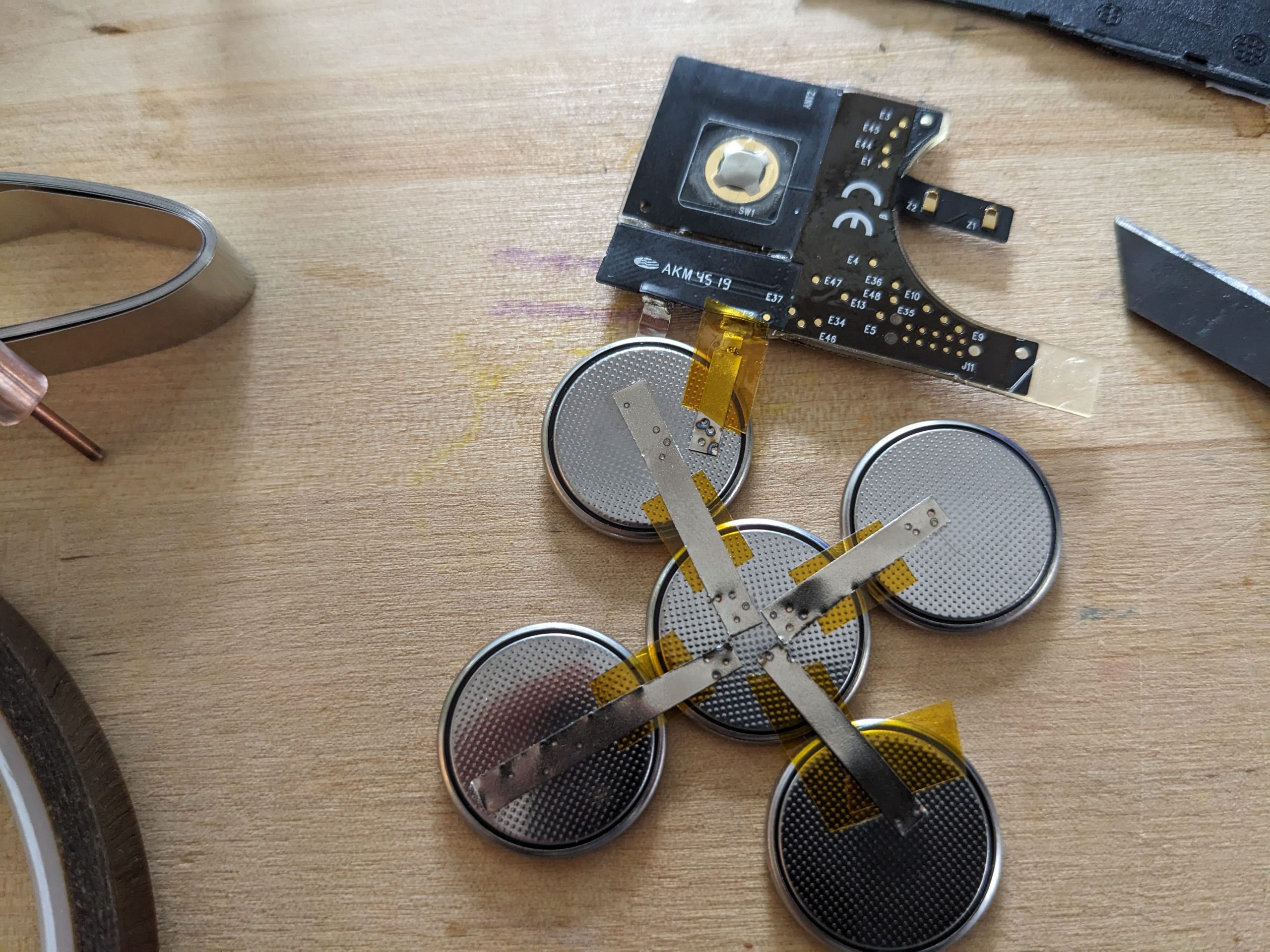
I had to add some little extensions to the tabs on the Tile board and then welded the batteries onto the tile board. Finally, a bit of packing tape closes the case back up! I could glue it back together but seems like a pain to undo in a couple years when the batteries need to be replaced again.

1/9